Usage¶

VectorBT allows you to easily backtest strategies with a couple of lines of Python code.

Examples¶

Invest $100 in Bitcoin since 2014¶

>>> import vectorbt as vbt

>>> data = vbt.YFData.download("BTC-USD")
>>> price = data.get("Close")

>>> pf = vbt.Portfolio.from_holding(price, init_cash=100)
>>> print(pf.total_profit())
19501.10906763755

Trade a dual-SMA crossover strategy¶

>>> fast_ma = vbt.MA.run(price, 10)
>>> slow_ma = vbt.MA.run(price, 50)
>>> entries = fast_ma.ma_crossed_above(slow_ma)
>>> exits = fast_ma.ma_crossed_below(slow_ma)

>>> pf = vbt.Portfolio.from_signals(price, entries, exits, init_cash=100)
>>> print(pf.total_profit())
34417.80960086067

VectorBT PRO

Simulate limit orders, use leverage, and model futures with contract multipliers.

Generate 1,000 random strategies¶

>>> import numpy as np

>>> symbols = ["BTC-USD", "ETH-USD"]
>>> data = vbt.YFData.download(symbols, missing_index="drop")
>>> price = data.get("Close")

>>> n = np.random.randint(10, 101, size=1000).tolist()
>>> pf = vbt.Portfolio.from_random_signals(price, n=n, init_cash=100, seed=42)

>>> mean_expectancy = pf.trades.expectancy().groupby(["randnx_n", "symbol"]).mean()
>>> fig = mean_expectancy.unstack().vbt.scatterplot(xaxis_title="randnx_n", yaxis_title="mean_expectancy")
>>> fig.show()

Test 10,000 dual-SMA window combinations¶

>>> symbols = ["BTC-USD", "ETH-USD", "XRP-USD"]
>>> data = vbt.YFData.download(symbols, missing_index="drop")
>>> price = data.get("Close")

>>> windows = np.arange(2, 101)
>>> fast_ma, slow_ma = vbt.MA.run_combs(price, window=windows, r=2, short_names=["fast", "slow"])
>>> entries = fast_ma.ma_crossed_above(slow_ma)
>>> exits = fast_ma.ma_crossed_below(slow_ma)

>>> pf = vbt.Portfolio.from_signals(price, entries, exits, size=np.inf, fees=0.001, freq="1D")

>>> fig = pf.total_return().vbt.heatmap(
...     x_level="fast_window", y_level="slow_window", slider_level="symbol", symmetric=True,
...     trace_kwargs=dict(colorbar=dict(title="Total return", tickformat="%")))
>>> fig.show()

VectorBT PRO

Use random search to sample a large parameter grid, or conditional parameters to exclude combinations such as a fast MA window longer than the slow MA window. The cross-validation tutorial shows how to select parameters on training data and evaluate them on later periods.

Inspect any strategy configuration¶

Digging into each strategy configuration is as simple as indexing with pandas:

>>> print(pf[(10, 20, "ETH-USD")].stats())
Start                          2017-11-09 00:00:00+00:00
End                            2026-01-03 00:00:00+00:00
Period                                2978 days 00:00:00
Start Value                                        100.0
End Value                                    1604.093789
Total Return [%]                             1504.093789
Benchmark Return [%]                          866.094127
Max Gross Exposure [%]                             100.0
Total Fees Paid                               204.226289
Max Drawdown [%]                               70.734951
Max Drawdown Duration                 1095 days 00:00:00
Total Trades                                          81
Total Closed Trades                                   80
Total Open Trades                                      1
Open Trade PnL                                -14.232533
Win Rate [%]                                       41.25
Best Trade [%]                                120.511071
Worst Trade [%]                               -27.772271
Avg Winning Trade [%]                          27.265519
Avg Losing Trade [%]                           -9.022864
Avg Winning Trade Duration    32 days 20:21:49.090909091
Avg Losing Trade Duration      8 days 16:51:03.829787234
Profit Factor                                   1.275515
Expectancy                                     18.979079
Sharpe Ratio                                    0.861945
Calmar Ratio                                    0.572758
Omega Ratio                                      1.20277
Sortino Ratio                                   1.301377
Name: (10, 20, ETH-USD), dtype: object

Plot any strategy configuration¶

>>> pf[(10, 20, "ETH-USD")].plot().show()

Animate Bollinger Bands across multiple symbols¶

VectorBT goes beyond backtesting, with tools for financial data analysis and visualization:

>>> symbols = ["BTC-USD", "ETH-USD", "XRP-USD"]
>>> data = vbt.YFData.download(symbols, period="6mo", missing_index="drop")
>>> price = data.get("Close")
>>> bbands = vbt.BBANDS.run(price)

>>> def plot(index, bbands):
...     bbands = bbands.loc[index]
...     fig = vbt.make_subplots(
...         rows=2, cols=1, shared_xaxes=True, vertical_spacing=0.15,
...         subplot_titles=("%B", "Bandwidth"))
...     fig.update_layout(showlegend=False, width=750, height=400)
...     bbands.percent_b.vbt.ts_heatmap(
...         trace_kwargs=dict(zmin=0, zmid=0.5, zmax=1, colorscale="Spectral", colorbar=dict(
...             y=(fig.layout.yaxis.domain[0] + fig.layout.yaxis.domain[1]) / 2, len=0.5
...         )), add_trace_kwargs=dict(row=1, col=1), fig=fig)
...     bbands.bandwidth.vbt.ts_heatmap(
...         trace_kwargs=dict(colorbar=dict(
...             y=(fig.layout.yaxis2.domain[0] + fig.layout.yaxis2.domain[1]) / 2, len=0.5
...         )), add_trace_kwargs=dict(row=2, col=1), fig=fig)
...     return fig

>>> vbt.save_animation("bbands.gif", bbands.wrapper.index, plot, bbands, delta=90, step=3, fps=3)
100%|██████████| 31/31 [00:21<00:00,  1.21it/s]

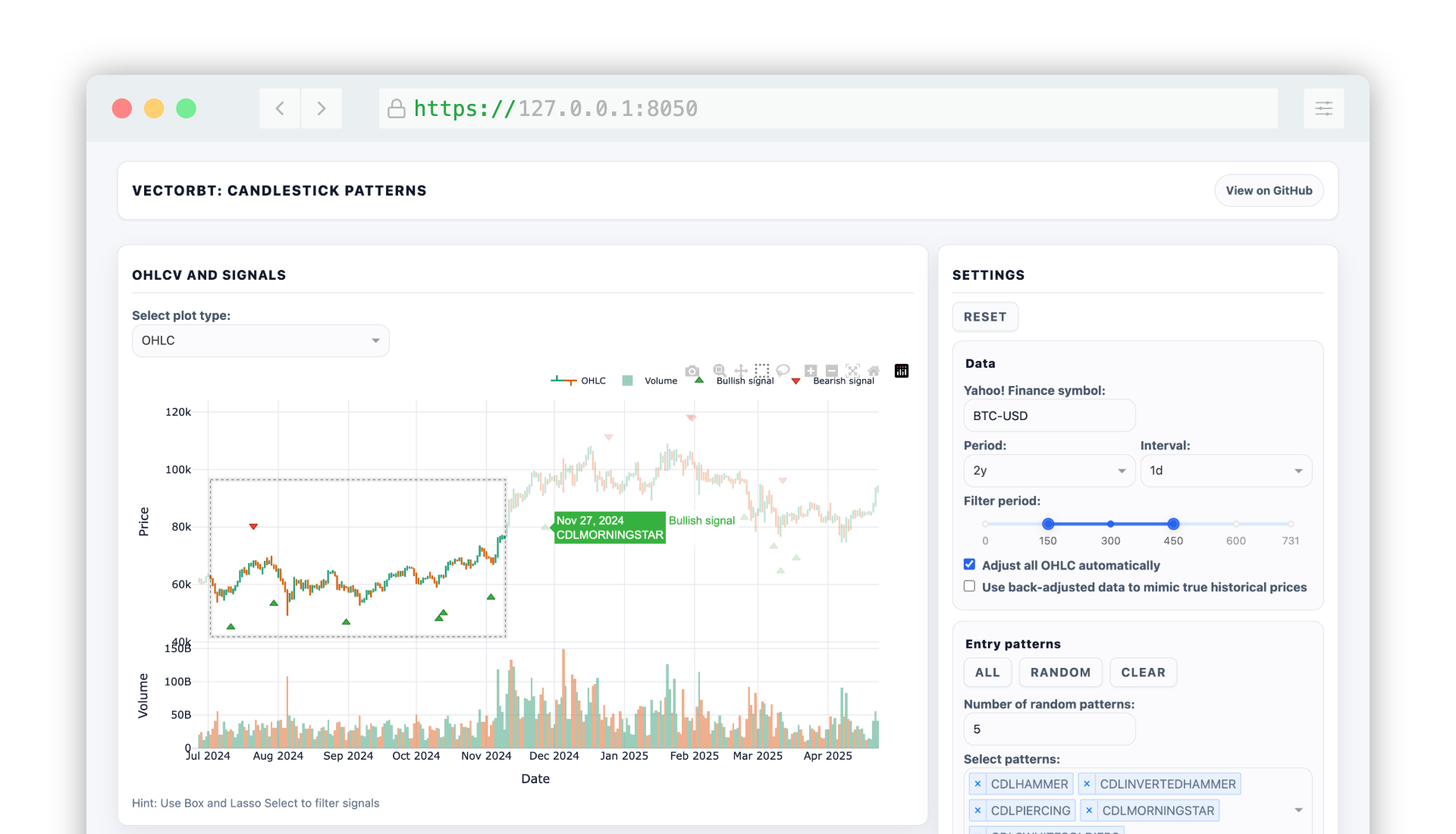
Example apps¶

Candlestick Patterns ¶

Explore candlestick patterns interactively and backtest their signals with VectorBT.

Learn more¶

See Resources for community examples and learning material. VectorBT vs PRO compares the editions. Browse the VectorBT PRO tutorials.