Features ¶

Pandas¶

Pandas acceleration: Compiled versions of most popular pandas functions, such as mapping, reducing, rolling, grouping, and resamping. For best performance, most operations are done strictly using NumPy and Numba. Attaches a custom accessor on top of pandas to easily switch between pandas and vectorbt functionality.

Compute the rolling z-score

>>> import vectorbt as vbt
>>> import pandas as pd
>>> import numpy as np
>>> from numba import njit

>>> big_ts = pd.DataFrame(np.random.uniform(size=(1000, 1000)))

# pandas
>>> @njit
... def zscore_nb(x):
...     return (x[-1] - np.mean(x)) / np.std(x)

>>> %timeit big_ts.rolling(2).apply(zscore_nb, raw=True)
482 ms ± 393 µs per loop (mean ± std. dev. of 7 runs, 1 loop each)

# vectorbt
>>> @njit
... def vbt_zscore_nb(i, col, x):
...     return zscore_nb(x)

>>> %timeit big_ts.vbt.rolling_apply(2, vbt_zscore_nb)
33.1 ms ± 1.17 ms per loop (mean ± std. dev. of 7 runs, 1 loop each)

Flexible broadcasting: Mechanism for broadcasting array-like objects of arbitrary shapes, including pandas objects with MultiIndex.

Broadcast pandas objects properly

>>> sr = pd.Series([1, 2, 3], index=['x', 'y', 'z'])
>>> df = pd.DataFrame([[4, 5, 6]], index=['x', 'y', 'z'], columns=['a', 'b', 'c'])

# pandas
>>> sr + df
    a   b   c   x   y   z
x NaN NaN NaN NaN NaN NaN
y NaN NaN NaN NaN NaN NaN
z NaN NaN NaN NaN NaN NaN

# vectorbt
>>> sr.vbt + df
   a  b  c
x  5  6  7
y  6  7  8
z  7  8  9

Pandas utilities: Grouping columns, wrapping NumPy arrays, transforming pandas objects and their indexes, and more.

Build a symmetric matrix

>>> pd.Series([1, 2, 3]).vbt.make_symmetric()
     0    1    2
0  1.0  2.0  3.0
1  2.0  NaN  NaN
2  3.0  NaN  NaN

Data¶

Data acquisition: Supports various data providers, such as Yahoo Finance, Binance, CCXT and Alpaca. Can merge multiple symbols with different index, as well as update them.

Download Alpaca data

>>> alpaca_data = vbt.AlpacaData.download(
...     "AAPL",
...     start='2 hours ago UTC',
...     end='15 minutes ago UTC',
...     interval='1m'
... )
>>> alpaca_data.get()
                           Open      High       Low     Close      Volume
timestamp                                                                
2021-12-27 14:04:00+00:00  177.0500  177.0500  177.0500  177.0500    1967
2021-12-27 14:05:00+00:00  177.0500  177.0500  177.0300  177.0500    3218
2021-12-27 14:06:00+00:00  177.0400  177.0400  177.0400  177.0400     873
...                             ...       ...       ...       ...     ...
2021-12-27 15:46:00+00:00  177.9500  178.0000  177.8289  177.8850  162778
2021-12-27 15:47:00+00:00  177.8810  177.9600  177.8400  177.9515  123284
2021-12-27 15:48:00+00:00  177.9600  178.0500  177.9600  178.0100  159700

[105 rows x 5 columns]

Data generation: Supports various (random) data generators, such as GBM.

Generate random data using Geometric Brownian Motion

>>> gbm_data = vbt.GBMData.download(
...     list(range(5)),
...     start='2020-01-01',
...     end='2021-01-01'
... )
>>> gbm_data.plot(showlegend=False)

Scheduled data updates: Can periodically update any previously downloaded data.

Append random data every 5 seconds

>>> class MyDataUpdater(vbt.DataUpdater):
...     def update(self, count_limit=None):
...         prev_index_len = len(self.data.wrapper.index)
...         super().update()
...         new_index_len = len(self.data.wrapper.index)
...         print(f"Data updated with {new_index_len - prev_index_len} data points")

>>> data = vbt.GBMData.download('SYMBOL', start='1 minute ago', freq='1s')
>>> my_updater = MyDataUpdater(data)
>>> my_updater.update_every(5, 'seconds')
Data updated with 5 data points
Data updated with 5 data points
...

Data preparation: Transformation, rescaling, and normalization of data. Custom splitters for cross-validation. Supports Scikit-Learn splitters, such as for K-Folds cross-validation.

Split time series data

>>> from datetime import datetime, timedelta

>>> index = [datetime(2020, 1, 1) + timedelta(days=i) for i in range(10)]
>>> sr = pd.Series(np.arange(len(index)), index=index)
>>> sr.vbt.rolling_split(
...     window_len=5, 
...     set_lens=(1, 1), 
...     left_to_right=False, 
...     plot=True, 
...     trace_names=['train', 'valid', 'test'])

Labeling for ML: Discrete and continuous label generation for effective training of ML models.

Identify local extrema

>>> price = np.cumprod(np.random.uniform(-0.1, 0.1, size=100) + 1)
>>> vbt.LEXLB.run(price, 0.2, 0.2).plot()

Indicators¶

Technical indicators: Most popular technical indicators with full Numba support, including Moving Average, Bollinger Bands, RSI, Stochastic, MACD, and more. Out-of-the-box support for 99% indicators in Technical Analysis Library, Pandas TA, and TA-Lib thanks to built-in parsers. Each indicator is wrapped with the vectorbt's indicator engine and thus accepts arbitrary hyperparameter combinations - from arrays to Cartesian products.

Compute 2 moving averages at once

>>> price = pd.Series([1, 2, 3, 4, 5], dtype=float)

# built-in
>>> vbt.MA.run(price, [2, 3]).ma
ma_window    2    3
0          NaN  NaN
1          1.5  NaN
2          2.5  2.0
3          3.5  3.0
4          4.5  4.0

# ta support
>>> vbt.ta('SMAIndicator').run(price, [2, 3]).sma_indicator
smaindicator_window    2    3
0                    NaN  NaN
1                    1.5  NaN
2                    2.5  2.0
3                    3.5  3.0
4                    4.5  4.0

# pandas-ta support
>>> vbt.pandas_ta('SMA').run(price, [2, 3]).sma
sma_length    2    3
0           NaN  NaN
1           1.5  NaN
2           2.5  2.0
3           3.5  3.0
4           4.5  4.0

# TA-Lib support
>>> vbt.talib('SMA').run(price, [2, 3]).real
sma_timeperiod    2    3
0               NaN  NaN
1               1.5  NaN
2               2.5  2.0
3               3.5  3.0
4               4.5  4.0

Indicator factory: Sophisticated factory for building custom technical indicators of any complexity. Takes a function and does all the magic for you: generates an indicator skeleton that takes inputs and parameters of any shape and type, and runs the vectorbt's indicator engine. The easiest and most flexible way to create indicators you will find in open source.

Construct a random indicator

>>> @njit
... def apply_func_nb(input_shape, start, mu, sigma):
...     rand_returns = np.random.normal(mu, sigma, input_shape)
...     return start * vbt.nb.nancumprod_nb(rand_returns + 1)

>>> RandomInd = vbt.IndicatorFactory(
...     param_names=['start', 'mu', 'sigma'],
...     output_names=['output']
... ).from_apply_func(
...     apply_func_nb,
...     require_input_shape=True,
...     seed=42
... )

>>> RandomInd.run(5, [100, 200], [-0.01, 0.01], 0.01).output
custom_start        100         200
custom_mu         -0.01        0.01
custom_sigma       0.01        0.01
0             99.496714  201.531726
1             98.364179  206.729658
2             98.017630  210.383470
3             98.530292  211.499608
4             97.314277  214.762117

Signals¶

Signal analysis: Generation, mapping and reducing, ranking, and distribution analysis of entry and exit signals.

Measure each partition of True values

>>> mask_sr = pd.Series([True, True, True, False, True, True])
>>> mask_sr.vbt.signals.partition_ranges().duration.values
array([3, 2])

Signal generators: Random and stop loss (SL, TSL, TP, etc.) signal generators with full Numba support.

Generate entries and exits using different probabilities

>>> rprobnx = vbt.RPROBNX.run(
...     input_shape=(5,),
...     entry_prob=[0.5, 1.],
...     exit_prob=[0.5, 1.],
...     param_product=True,
...     seed=42)

>>> rprobnx.entries
rprobnx_entry_prob    0.5    0.5    1.0    0.5
rprobnx_exit_prob     0.5    1.0    0.5    1.0
0                    True   True   True   True
1                   False  False  False  False
2                   False  False  False   True
3                   False  False  False  False
4                   False  False   True   True

>>> rprobnx.exits
rprobnx_entry_prob    0.5    0.5    1.0    1.0
rprobnx_exit_prob     0.5    1.0    0.5    1.0
0                   False  False  False  False
1                   False   True  False   True
2                   False  False  False  False
3                   False  False   True   True
4                    True  False  False  False

Signal factory: Signal factory based on indicator factory specialized for iterative signal generation.

Place entries and exits using custom functions

>>> @njit
... def entry_choice_func(from_i, to_i, col):
...     return np.array([col])

>>> @njit
... def exit_choice_func(from_i, to_i, col):
...     return np.array([to_i - 1])

>>> MySignals = vbt.SignalFactory().from_choice_func(
...     entry_choice_func=entry_choice_func,
...     exit_choice_func=exit_choice_func,
...     entry_kwargs=dict(wait=1),
...     exit_kwargs=dict(wait=0)
... )

>>> my_sig = MySignals.run(input_shape=(3, 3))
>>> my_sig.entries
       0      1      2
0   True  False  False
1  False   True  False
2  False  False   True
>>> my_sig.exits
       0      1      2
0  False  False  False
1  False  False  False
2   True   True   True

Modeling¶

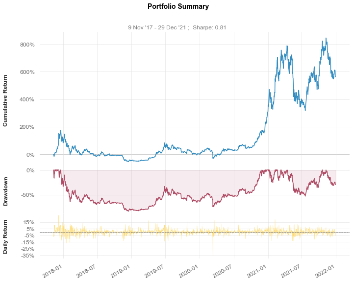
Portfolio modeling: The fastest backtesting engine in open source: fills 1,000,000 orders in 70-100ms on Apple M1. Flexible and powerful simulation functions for portfolio modeling, highly optimized for highest performance and lowest memory footprint. Supports two major simulation modes: 1) vectorized backtesting using user-provided arrays, such as orders, signals, and records, and 2) event-driven backtesting using user-defined callbacks. Supports shorting and individual as well as multi-asset mixed portfolios. Combines many features across vectorbt into a single behemoth class.

Backtest the Golden Cross

>>> price = vbt.YFData.download('BTC-USD', start='2018-01-01').get('Close')
>>> fast_ma = vbt.MA.run(price, 50, short_name='fast_ma')
>>> slow_ma = vbt.MA.run(price, 200, short_name='slow_ma')
>>> entries = fast_ma.ma_crossed_above(slow_ma)
>>> exits = fast_ma.ma_crossed_below(slow_ma)
>>> pf = vbt.Portfolio.from_signals(price, entries, exits, fees=0.005)

>>> pf.orders.records_readable
   Order Id  Column                 Timestamp      Size         Price  \\
0         0       0 2019-04-24 00:00:00+00:00  0.018208   5464.866699   
1         1       0 2019-10-26 00:00:00+00:00  0.018208   9244.972656   
2         2       0 2020-02-19 00:00:00+00:00  0.017300   9633.386719   
3         3       0 2020-03-25 00:00:00+00:00  0.017300   6681.062988   
4         4       0 2020-05-21 00:00:00+00:00  0.012600   9081.761719   
5         5       0 2021-06-19 00:00:00+00:00  0.012600  35615.871094   
6         6       0 2021-09-15 00:00:00+00:00  0.009222  48176.347656   

       Fees  Side  
0  0.497512   Buy  
1  0.841647  Sell  
2  0.833272   Buy  
3  0.577901  Sell  
4  0.572151   Buy  
5  2.243800  Sell  
6  2.221473   Buy  

>>> fig = price.vbt.plot(trace_kwargs=dict(name='Close'))
>>> fast_ma.ma.vbt.plot(trace_kwargs=dict(name='Fast MA'), fig=fig)
>>> slow_ma.ma.vbt.plot(trace_kwargs=dict(name='Slow MA'), fig=fig)
>>> pf.positions.plot(close_trace_kwargs=dict(visible=False), fig=fig)

Analysis¶

Performance metrics: Numba-compiled versions of metrics from empyrical and their rolling versions. Adapter for QuantStats.

Visualize performance using QuantStats

>>> price = vbt.YFData.download('BTC-USD').get('Close')
>>> returns = price.vbt.to_returns()
>>> returns.vbt.returns.qs.plot_snapshot()

Stats builder: Class for building statistics out of custom metrics. Implements a preset of tailored statistics for many backtesting components, such as signals, returns, and portfolio.

Analyze the distribution of signals in a mask

>>> index = [datetime(2020, 1, 1) + timedelta(days=i) for i in range(7)]
>>> mask = pd.Series([False, True, True, True, False, True, False])
>>> mask.vbt.signals(freq='d').stats()
Start                                               0
End                                                 6
Period                                7 days 00:00:00
Total                                               4
Rate [%]                                    57.142857
First Index                                         1
Last Index                                          5
Norm Avg Index [-1, 1]                      -0.083333
Distance: Min                         1 days 00:00:00
Distance: Max                         2 days 00:00:00
Distance: Mean                        1 days 08:00:00
Distance: Std               0 days 13:51:23.063257983
Total Partitions                                    2
Partition Rate [%]                               50.0
Partition Length: Min                 1 days 00:00:00
Partition Length: Max                 3 days 00:00:00
Partition Length: Mean                2 days 00:00:00
Partition Length: Std       1 days 09:56:28.051789035
Partition Distance: Min               2 days 00:00:00
Partition Distance: Max               2 days 00:00:00
Partition Distance: Mean              2 days 00:00:00
Partition Distance: Std                           NaT
dtype: object

Records and mapped arrays: In-house data structures for analyzing complex data, such as simulation logs. Fully compiled with Numba.

Parse 5 highest slippage values from logs

>>> price = vbt.YFData.download('BTC-USD').get('Close')
>>> slippage = np.random.uniform(0, 0.005, size=price.shape[0])
>>> logs = vbt.Portfolio.from_random_signals(price, n=5, slippage=slippage, log=True).logs

>>> req_price_ma = logs.map_field('req_price')
>>> res_price_ma = logs.map_field('res_price')
>>> slippage_ma = (res_price_ma - req_price_ma) / req_price_ma
>>> slippage_ma = slippage_ma.replace(arr=np.abs(slippage_ma.values))
>>> top_slippage_pd = slippage_ma.top_n(5).to_pd()
>>> top_slippage_pd[~top_slippage_pd.isnull()]
Date
2017-12-25 00:00:00+00:00    0.001534
2018-06-03 00:00:00+00:00    0.004354
2018-12-03 00:00:00+00:00    0.004663
2019-09-20 00:00:00+00:00    0.004217
2020-11-28 00:00:00+00:00    0.000775
dtype: float64

Trade analysis: Retrospective analysis of trades from various view points. Supports entry trades, exit trades, and positions.

Get the projected return of each buy order

>>> price = vbt.YFData.download('BTC-USD').get('Close')
>>> entry_trades = vbt.Portfolio.from_random_signals(price, n=5).entry_trades
>>> returns_pd = entry_trades.returns.to_pd()
>>> returns_pd[~returns_pd.isnull()]
Date
2017-11-12 00:00:00+00:00    0.742975
2019-08-30 00:00:00+00:00   -0.081744
2020-04-21 00:00:00+00:00    0.489072
2020-09-13 00:00:00+00:00    0.262251
2021-03-07 00:00:00+00:00   -0.382155
dtype: float64

Drawdown analysis: Drawdown statistics of any numeric time series.

Plot 3 deepest price dips

>>> price = vbt.YFData.download('BTC-USD').get('Close')
>>> price.vbt.drawdowns.plot(top_n=3)

Plotting¶

Data visualization: Numerous flexible data plotting functions distributed across vectorbt.

Plot time series against each other

>>> sr1 = pd.Series(np.cumprod(np.random.normal(0, 0.01, 100) + 1))
>>> sr2 = pd.Series(np.cumprod(np.random.normal(0, 0.01, 100) + 1))
>>> sr1.vbt.plot_against(sr2)

Figures and widgets: Custom interactive figures and widgets using Plotly, such as Heatmap and Volume. All custom widgets have dedicated methods for efficiently updating their state.

Plot a volume

>>> volume_widget = vbt.plotting.Volume(
...     data=np.random.randint(1, 10, size=(3, 3, 3)),
...     x_labels=['a', 'b', 'c'],
...     y_labels=['d', 'e', 'f'],
...     z_labels=['g', 'h', 'i']
... )
>>> volume_widget.fig

Plots builder: Class for building plots out of custom subplots. Implements a preset of tailored subplots for many backtesting components, such as signals, returns, and portfolio.

Plot various portfolio balances

>>> price = vbt.YFData.download('BTC-USD').get('Close')
>>> pf = vbt.Portfolio.from_random_signals(price, n=5)
>>> pf.plot(subplots=['cash', 'assets', 'value']).show_svg()

Extra¶

Notifications: Telegram bot based on Python Telegram Bot.

Launch a bot that returns the latest ticker on Binance

>>> from telegram.ext import CommandHandler
>>> import ccxt

>>> class BinanceTickerBot(vbt.TelegramBot):
...     @property
...     def custom_handlers(self):
...         return CommandHandler('get', self.get),
...
...     @property
...     def help_message(self):
...         return "Type /get [symbol] to get the latest ticker on Binance."
...
...     def get(self, update, context):
...         chat_id = update.effective_chat.id
...         try:
...             ticker = ccxt.binance().fetchTicker(context.args[0])
...         except Exception as e:
...             self.send_message(chat_id, str(e))
...             return
...         self.send_message(chat_id, str(ticker['last']))

>>> bot = BinanceTickerBot(token='YOUR_TOKEN')
>>> bot.start()

General utilities: Scheduling using schedule, templates, decorators, configs, and more.

Every 10 seconds display the latest Bitcoin trades on Binance

>>> from vectorbt.utils.datetime_ import datetime_to_ms, to_tzaware_datetime, get_utc_tz
>>> from IPython.display import SVG, display, clear_output

>>> exchange = ccxt.binance()

>>> def job_func():
...     since = datetime_to_ms(to_tzaware_datetime('10 seconds ago UTC', tz=get_utc_tz()))
...     trades = exchange.fetch_trades('BTC/USDT', since)
...     price = pd.Series({t['datetime']: t['price'] for t in trades})
...     svg = price.vbt.plot().to_image(format="svg")
...     clear_output()
...     display(SVG(svg))

>>> scheduler = vbt.ScheduleManager()
>>> scheduler.every(10, 'seconds').do(job_func)
>>> scheduler.start()

Caching: Property and method decorators for caching most frequently used objects.

Create a cached method and disable it globally

>>> import time
>>> start = time.time()

>>> class MyClass:
...     @vbt.cached_method
...     def get_elapsed(self):
...         return time.time() - start

>>> my_inst = MyClass()
>>> my_inst.get_elapsed()
0.00010895729064941406

>>> my_inst.get_elapsed()
0.00010895729064941406

>>> get_elapsed_cond = vbt.CacheCondition(instance=my_inst, func='get_elapsed')
>>> vbt.settings.caching['blacklist'].append(get_elapsed_cond)
>>> my_inst.get_elapsed()
0.01081395149230957

Persistance: Most Python objects including data and portfolio can be saved to a file and retrieved back using Dill.

Simulate, save, and load back a portfolio

>>> price = vbt.YFData.download('BTC-USD').get('Close')
>>> pf = vbt.Portfolio.from_random_signals(price, n=5)
>>> pf.save('my_pf.pkl')

>>> pf = vbt.Portfolio.load('my_pf.pkl')
>>> pf.total_return()
5.96813681074424